Spectroscopy Advanced

How to Interpret the Reported Matches

There are several important things to consider when interpreting a spectral match including the library source, the Pearson’s r, and other metrics.

The Library Source

When you click on a spectrum, all of the metadata that we have in Open Specy about that source will be displayed in a metadata window below to the matches table. Each library has different methodologies used to develop it. It is useful to read up on the library sources from the literature that they came from. E.g. Chabuka et al. 2020 focuses on weathered plastics, so matching to it may suggest that your spectrum is of a weathered polymer. Primpke et al. 2018 only has a spectral range up to 2000, so some polymers may be difficult to differentiate with it. Make sure to cite the libraries that you use during your search when you publish your results. The authors were kind enough to make their data open access so that it could be used in Open Specy and we should return the favor by citing them.

Compact In-Memory Spectra

For advanced map and repeated-spectrum work, Specs can retain spectra in memory while compacting regular coordinates and repeated metadata. Dense OpenSpecy remains the default for read_envi() and read_h5(); request representation = "Specs" explicitly. An optional background policy is lossy: it maps rejected or non-finite pixels to an exact-zero virtual spectrum and records that decision. Coordinate and repeated-metadata compaction is lossless.

policy <- specs_background_filter(
  metric = "run_sig_over_noise", minimum = 4, sigma = c(1, 1, 1)
)
map <- read_envi(
  "map.dat", "map.hdr", representation = "Specs",
  background_filter = policy, spectral_smooth = TRUE
)
specs_background_mask(map)
decompress_spec(map, index = 1)

PCA, weighted Lloyd K-means, and Hilbert encoding remain explicit full-object transformations. Background spectra keep code or class zero and are excluded from fitting. Use one fitted PCA/Hilbert model for both reference and query objects so their codes share the same limits.

model <- fit_specs_pca(spec_lib, n_components = 16)
library_specs <- as_Specs(spec_lib, model)
query_specs <- as_Specs(
  raman_proc, model, limits = attr(library_specs, "hilbert_model")
)
match_spec(query_specs, library_specs, top_n = 5)

For a large in-memory OpenSpecy query, bound the temporary reference-by-query correlation matrix with batch_size. A smaller positive integer lowers peak memory and adds loop overhead; a larger value is faster when memory permits. Bounded matching requires a finite top_n and preserves the same ranked rows and ordering as the dense calculation.

matches <- match_spec(
  query_map, library = spec_lib, top_n = 1, batch_size = 1000
)

The file-backed FileSpecs workflow for maps larger than memory is documented in the standard operating procedure. The bundled and browser app pipeline, including spatial and spectral clustering behavior, is documented in the app vignette.

Pearson’s r

Correlation values are used to identify the closest matches available in the current Open Specy spectral libraries to improve material identification and reduce sample processing times. Pearson’s r values range from 0 - 1 with 0 being a completely different spectrum and 1 being an exact match. Some general guidelines that we have observed from using Open Specy. If no matches are > ~0.6 the material may require additional processing or may not exist in the Open Specy library. Correlation values are not the only metric you should use to assess your spectra’s match to a material in the library, matches need to make sense.

Things to Consider beyond Correlation

Peak position and height similarities are more important than correlation and need to be assessed manually. Peak position correlates with specific bond types. Peak height correlates to the concentration of a compound. Therefore, peak height and peak position should match as closely as possible to the matched spectrum. When there are peaks that exist in the spectra you are trying to interpret that do not exist in the match, there may be additional materials to identify. In this case, restrict the processing range to just the unidentified peak and try to identify it as an additional component (see also https://www.compoundchem.com/2015/02/05/irspectroscopy/).

Also, check the match metadata to see if the match makes sense. Example: A single fiber cannot be a “cotton blend” since there would be no other fibers to make up the rest of the blend. Example: Cellophane does not degrade into fibers, so a match for a fiber to cellophane wouldn’t make sense. Example: You are analyzing a particle at room temperature, but the matched material is liquid at room temperature. The material may be a component of the particle but it cannot be the whole particle.

How Specific Do You Need to be in the Material Type of the Match?

You can choose to be specific about how you classify a substance (e.g. polyester, cellophane) or more general (e.g. synthetic, semi-synthetic, natural, etc.). The choice depends on your research question. Using more general groups can speed up analysis time but will decrease the information you have for interpretation. To identify materials more generally, you can often clump the identities provided by Open Specy to suit your needs. For example, matches to “polyester” and “polypropylene” could be clumped to the category “plastic”.

How to Differentiate Between Similar Spectra?

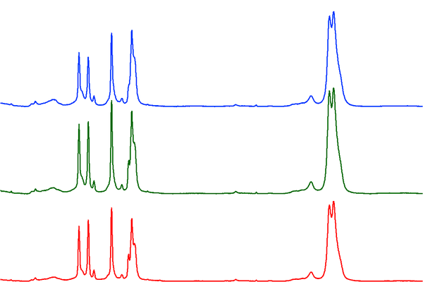
One common challenge is differentiating between LDPE and HDPE. But, even with a low resolution instrument (MacroRAM, 2 cm^-1 pixel^-1), you can still see some differences. From a wide view, these low, medium, and high density PE samples all look relatively similar (figures courtesy of Bridget O'Donnell, Horiba Scientific):

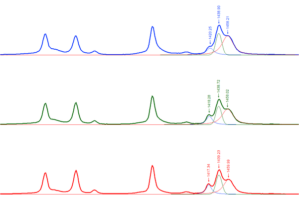
But, a closer look at the 1450 cm^-1 band reveals clear differences:

When you overlay them, you start to see differences in other spectral regions too:

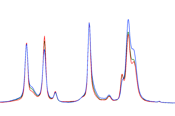
So, the question is, how do we deal with samples that are very similar with only subtle differences? Usually, researchers will use MVA techniques after they’ve collected multiple reference spectra of known samples (LDPE and HDPE in this case). They can then develop models and apply them to distinguish between different types of PE. With a reference database like Open Specy, this is complicated by the fact that researchers are measuring samples on different instruments with correspondingly different spectral responses and spectral resolutions. That makes it even more difficult to accurately match definitively to LDPE and HDPE as opposed to generic ‘PE’.

One possibility is to place more emphasis (from a computational perspective) on the bands that show the most difference (the triplet at 1450 cm^-1) by restricting the range used to match in Open Specy.

The other, much simpler option is to just match any PE hit to generic ‘PE’ and not specifically HDPE or LDPE.

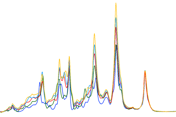
Another challenge is in differentiating between types of nylons. But, Raman has a pretty easy time distinguishing nylons. These spectra were recorded of a series of nylons and the differences are much more distinguishable compared to the PE results above (nylon 6, 6-6, 6-9, 6-10, and 6-12 top to bottom):

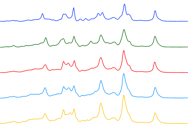
The differences are even more pronounced when you overlay the spectra:

What to Do When Matches Aren’t Making Sense

Double check that the baseline correction and smoothing parameters result in the best processing of the data.
Try reprocessing your spectrum, but limit it to specific peak regions with a higher signal to noise ratio.
Restrict the spectral range to include or exclude questionable peaks or peaks that were not present in the previous matches.
Restrict the spectral range to exclude things like CO₂ (2200 cm^-1) or H₂O (~1600 cm^-1) in spikes in the IR spectrum.
If nothing above works to determine a quality match, you may need to measure the spectrum of your material again or use another spectral analysis tool.

Experimental Temperature and Emissivity Diagnostics

estimate_temperature() and calculate_emissivity() apply only to calibrated FTIR surface-leaving spectral radiance in W m^-2 sr^-1 (cm^-1)^-1. They do not convert absorbance, transmittance, reflectance, normalized spectra, derivatives, baseline-corrected spectra, or arbitrary detector counts into radiance. Set the object’s spectra_type to "ftir" and its intensity_unit to the exact radiance unit, and retain traceable calibration and surface-leaving provenance in its metadata. A unit label is a declaration about upstream calibration, not proof that calibration was performed.

The experimental retrieval models an opaque, isothermal surface as

$L = \epsilon B(T) + (1 - \epsilon)L_{down},$

where $L$ is measured surface-leaving radiance, $B(T)$ is Planck radiance at temperature $T$ , $L_{down}$ is environmental downwelling radiance, and $\epsilon$ is effective emissivity. The Planck calculation follows the NIST wavenumber formulation. Temperature-emissivity separation is underdetermined; this implementation uses the spectral-smoothness premise described by Borel, so the result is model-conditioned rather than an independent thermometric measurement.

Three physical inputs must be chosen for each acquisition:

downwelling is measured or modelled environmental radiance in the same units and on the same bands as the map. A scalar zero is accepted only as an explicit no-background assumption; it is not a safe general default.
temperature_range_k is a physically defensible lower and upper bound in Kelvin. Too narrow a range rejects a real solution at a boundary; an unnecessarily broad range increases ambiguity and computation.
fit_range_cm1 restricts the fit to a calibrated, usable thermal-emission interval in cm^-1. Exclude saturated, poorly calibrated, and strong atmospheric-interference bands. For targets near room temperature, use a validated longwave interval. The 3–5 micrometre region can require reflected-source, solar, and directional-reflectance terms that this model does not include; see Cheng et al..

If radiance uncertainty is available, pass it with radiance_uncertainty in the same radiance units. Larger uncertainty causes more channels to be treated as uninformative or near-singular. Without it, numerical safeguards can detect unstable denominators but cannot quantify measurement uncertainty.

Efficient Map-Level Metrics

The standard in-memory OpenSpecy method is optimized for large maps. It searches spectra in bounded matrix blocks and returns one row per input spectrum instead of allocating a bands-by-pixels emissivity cube. Choose the single emissivity summary returned in emissivity_value:

"planck_weighted" (the default) is the band-integrated directional effective emissivity, $\sum_i \epsilon_i B_i(T)\Delta\widetilde{\nu}_i / \sum_i B_i(T)\Delta\widetilde{\nu}_i$ , over the selected fit bands;
"mean" summarizes the unweighted fitted emissivity level;
"median" is less sensitive to isolated bands and is often a useful robust map contrast; and
"max" emphasizes the highest fitted band but is most sensitive to noise, calibration errors, and out-of-range values.

The Planck-weighted value is limited to the measured wavenumber interval and viewing geometry. It is not a tabulated total hemispherical emissivity, which would require integration over the full relevant spectrum and emission angles. Wilber, Kratz, and Gupta, for example, form broadband emissivities from spectral values using the Planck energy distribution and report the band and assumed temperature.

For example, a 100,000-pixel in-memory map can be reduced to aligned scalar diagnostics without materializing 100,000 emissivity spectra:

thermal_metrics <- estimate_temperature(
  radiance_map,
  downwelling = measured_downwelling,
  temperature_range_k = c(290, 380),
  fit_range_cm1 = c(800, 1250),
  radiance_uncertainty = measured_uncertainty,
  emissivity_stat = "planck_weighted"
)

heatmap_spec(radiance_map, z = thermal_metrics$emissivity_value)

block_size = NULL chooses a bounded block automatically. A smaller positive whole number reduces transient memory at the cost of more block overhead; a larger value may be faster but uses more memory. It must not change numerical results. The FileSpecs method is available for file-backed acquisitions and uses the same kernel, but calibrated in-memory OpenSpecy maps are a primary optimized use case rather than a required conversion to disk.

The output remains in source order and includes estimated material temperature, the requested emissivity value, roughness, physical-range and valid-band fractions, and a fit status. Use only rows where status == "ok"; keep failed rows as NA. Boundary, flat, multiple-minimum, near-singular, and insufficient-band outcomes are rejections, not extreme particle values. Emissivity is deliberately not clipped to 0–1: values outside that interval can expose calibration, background, mixing, or model failure. There is no universal rule that higher or lower emissivity indicates a particle, so any predicate passed to def_features() must be validated for that acquisition.

Compare the temperature/emissivity metric on held-out labelled pixels against direct radiance contrast and an appropriate signal-to-noise metric. Use it only when it adds reproducible separation. Where the assumptions of sig_noise() fit the acquisition, retain that result as a baseline rather than replacing it with emissivity. For example, after choosing a threshold from independent controls:

particle_pixels <- thermal_metrics$status == "ok" &
  thermal_metrics$emissivity_value > validated_threshold

particle_map <- def_features(radiance_map, features = particle_pixels) |>
  collapse_spec()

# Temperature is nonlinear: estimate it again after spectra are collapsed.
particle_metrics <- estimate_temperature(
  particle_map,
  downwelling = measured_downwelling,
  temperature_range_k = c(290, 380),
  fit_range_cm1 = c(800, 1250),
  emissivity_stat = "median"
)

# Materialize full curves only for collapsed particles with successful fits.
ok_particles <- particle_metrics$status == "ok"
particle_emissivity <- calculate_emissivity(
  filter_spec(particle_map, ok_particles),
  temperature_k =
    particle_metrics$estimated_material_temperature_k[ok_particles],
  downwelling = measured_downwelling
)

Use calculate_emissivity() only when full emissivity curves are needed for a small selected or collapsed set. Supply the corresponding fitted temperature and downwelling radiance. Thin, transmitting, scattering, subpixel-mixed, or non-isothermal particles yield effective pixel emissivity, not an intrinsic material constant. Do not pass the emissivity curves to process_spec() or match_spec(), and do not use them to overwrite a conventional FTIR spectrum collected for library identification. Keep identification and radiometric diagnostic workflows separate. Absolute smoothness can also produce false high-temperature minima, as demonstrated by Wu et al.; OpenSpecy therefore rejects ambiguous or boundary solutions instead of forcing an estimate.

References

Borel CC (1997). Iterative Retrieval of Surface Emissivity and Temperature for a Hyperspectral Sensor. Los Alamos National Laboratory report LA-UR-97-3012. https://digital.library.unt.edu/ark:/67531/metadc696880/.

Cheng J, Liang S, Wang J, Li X (2011). A Stepwise Refining Algorithm of Temperature and Emissivity Separation for Hyperspectral Thermal Infrared Data. IEEE Transactions on Geoscience and Remote Sensing, 49(5), 1588–1597. doi: 10.1109/TGRS.2010.2076818.

Chabuka BK, Kalivas JH (2020). “Application of a Hybrid Fusion Classification Process for Identification of Microplastics Based on Fourier Transform Infrared Spectroscopy.” Applied Spectroscopy, 74(9), 1167–1183. doi: 10.1177/0003702820923993.

Cowger W, Gray A, Christiansen SH, De Frond H, Deshpande AD, Hemabessiere L, Lee E, Mill L, et al. (2020). “Critical Review of Processing and Classification Techniques for Images and Spectra in Microplastic Research.” Applied Spectroscopy, 74(9), 989–1010. doi: 10.1177/0003702820929064.

Cowger W, Steinmetz Z, Gray A, Munno K, Lynch J, Hapich H, Primpke S, De Frond H, Rochman C, Herodotou O (2021). “Microplastic Spectral Classification Needs an Open Source Community: Open Specy to the Rescue!” Analytical Chemistry, 93(21), 7543–7548. doi: 10.1021/acs.analchem.1c00123.

Primpke S, Wirth M, Lorenz C, Gerdts G (2018). “Reference Database Design for the Automated Analysis of Microplastic Samples Based on Fourier Transform Infrared (FTIR) Spectroscopy.” Analytical and Bioanalytical Chemistry, 410(21), 5131–5141. doi: 10.1007/s00216-018-1156-x.

Renner G, Schmidt TC, Schram J (2017). “A New Chemometric Approach for Automatic Identification of Microplastics from Environmental Compartments Based on FT-IR Spectroscopy.” Analytical Chemistry, 89(22), 12045–12053. doi: 10.1021/acs.analchem.7b02472.

Richmond JC, Nicodemus FE (1985). “Blackbodies, Blackbody Radiation, and Temperature Scales.” In Self-Study Manual on Optical Radiation Measurements: Part I–Concepts, Chapter 12. National Bureau of Standards Technical Note 910-8. NIST publication record.

Wilber AC, Kratz DP, Gupta SK (1999). Surface Emissivity Maps for Use in Satellite Retrievals of Longwave Radiation. NASA/TP-1999-209362. https://ntrs.nasa.gov/citations/19990100634.

Savitzky A, Golay MJ (1964). “Smoothing and Differentiation of Data by Simplified Least Squares Procedures.” Analytical Chemistry, 36(8), 1627–1639.

Wu Z, Ren H, Zhang T, Qin Q, Dong J, Ye X (2017). “A Modified Method to Prevent False Minimums Occurring in Iterative Spectrally Smooth Temperature Emissivity Separation.” In 2017 IEEE International Geoscience and Remote Sensing Symposium (IGARSS), 6170–6173. doi: 10.1109/IGARSS.2017.8128417.

Zhao J, Lui H, McLean DI, Zeng H (2007). “Automated Autofluorescence Background Subtraction Algorithm for Biomedical Raman Spectroscopy.” Applied Spectroscopy, 61(11), 1225–1232. doi: 10.1366/000370207782597003.

2026-09-24